Introduction

The knowledge of the process of food degradation by the rumen microorganisms is important in studies on the evaluation of foods for ruminants, since the knowledge of the potential nutritional value of foods, by ruminal degradation, allows its rational employment as sole food or as ingredient in more complex mixtures^(1,2).

Food consumption is highly correlated with its nutritional composition and digestibility, since the physiological regulation occurs when there is the rise in dry matter consumption with the increase in digestibility, corroborating the animal's satiety^(3,4).

Among the techniques employed to evaluate the ruminal degradation of foods, the in situ technique has been the most extensively used, which consists in determining the disappearance of components from the sample of the foods stored in rumen-incubated nylon bags, for variable periods⁽⁵⁾. Although it does not allow the food to suffer all digestive events, such as chewing and rumination, according to Pereira et al.⁽⁶⁾, the extensive use of this technique is related to its fast and easy execution, since it requires a small amount of sample from the test food and enables its exposure to the ruminal environment, besides its results being close to those found with in vivo trial.

The nonlinear models are widely used in studies which aim at estimating the parameters of the kinetics of in situ ruminal degradation⁽⁷⁾. Nonetheless, given the large quantity of factors involved in the performance of these experiments, different procedures and models of analyses may be used^(6,8-12). Since these studies involve longitudinal data, as the degradation measures are systematically obtained over time in the same experimental units, it is expected that there is a nonzero correlation among the successive measures and heterogeneity of the variances among the measures performed on the different occasions. These aspects are not considered in the classical methods of estimation and of univariate analysis of variance, which may alter the results of the inferences made on the model parameters. Pasternak and Shalev⁽¹³⁾ affirmed that the simple adjustment of a nonlinear regression to longitudinal data might be inefficient, since it does not consider the heterogeneity of the variances. Sartorio⁽¹⁴⁾ and Carvalho et al.⁽¹⁵⁾, among others, affirmed that the traditional analysis of the data performed in two phases(5,8,9) must also be inefficient, since, besides not considering the heterogeneity of the variances, it does not consider the possible correlation among the measurements repeated over time, which hurts the premise of sphericity of the structure of variances and covariances, which is a demand of the classical regression models. A later approach for the analysis of longitudinal data with nonlinear behavior for the medium responses involves the use of mixed nonlinear models (MNLM), which are still little employed in the analysis of ruminal degradability trials⁽¹⁴⁾. In view of the above, the aim of this work is to present and evaluate the applicability of mixed nonlinear models to describe the kinetics of in situ ruminal degradation of Tifton 85 hays, in steers fed diets composed of different combinations of roughage:concentrate and hay from two different nutritional qualities, comparing their results with those obtained in the traditional analysis, which is performed in two phases.

Materials and methods

The data were obtained from the experiment developed by Feitosa et al.⁽¹⁷⁾, at the Animal Unit for Digestive and Metabolic Studies of the Departamento de Zootecnia da Faculdade de Ciências Agrárias e Veterinárias/UNESP, Jaboticabal Campus, in the period from May 2001 to December 2002.

Six ruminally cannulated crossbred steers (Bos taurus × Bos taurus indicus) were used, with average weight of 550±35kg and approximately three and a half years old. During the experimental period, the animals were maintained in individual stalls, provided with water trough and feeder, receiving diets composed of Tifton 85 (TIF) hay and concentrate in two daily meals, at 7h30 and at 18h30. The amount of food provided was based on the maximum daily consumption verified with the diet with the highest roughage percentage and the worst nutritional quality. The animals were adapted to the treatments for 14 days, followed by 10 days of sample collection for each experimental period.

The six feeds prepared were composed of the combination of three different ratios, 70:30, 50:50 and 30:70 of roughage (R) and concentrate (C), based on the dry matter, and two Tifton 85 hays with 4% (TIF4) and 10% (TIF10) of crude protein, both minced into 5 mm particles. The concentrate was composed of soybean (Glycine max L.) hull, ground corn (Zea mays L.) and sunflower (Helianthus annuus L.) bran. The treatments were identified as: R70TIF4, R70TIF10, R50TIF4, R50TIF10, R30TIF4 and R30TIF10.

The ruminal degradability of the dry matter (DM) was determined by the in situ technique, using bags made of nylon, measuring approximately 14×7 cm, with pores of 50µm, containing samples of each of the experimental diets milled with granulometry of 5 mm. 4.5 g of sample (base on DM) were incubated, tied to links of a steel chain for all incubation times. The ten incubation times in the rumen were of 120, 96, 84, 72, 60, 48, 24, 12, 6 and 3 hours with two replicates for each time and animal, adopting the nylon bag placem changing the water of the machine every five minutes ent system at the incubation times and the simultaneous removal of all bags at the end of the period.

After incubation, the nylon bags were pre-washed in running water for the removal of the excess of ruminal content and placed in water with ice for 20 min. Subsequently, they were washed for 15 minutes in a washing machine without centrifugation (changing the water of the machine every five minutes). After this step, the bags with the residues were dried in an oven at 65 °C, with forced air circulation for 48 hours.

The bags with the dry residues were weighed and their residues were ground in a knife mill, with a sieve of 1mm in diameter, stored in bottles with lid and identified. The samples were dried in an oven regulated at 105 oC for 12 hours and the analyses to determine the dry matter were performed at the Laboratório de Ingredientes e Gases Poluentes (LIGAP) of the Departamento de Zootecnia da FCAV/UNESP, Jaboticabal Campus – SP.

The basic experiment was planned in a 6×6 latin square with six animals at six distinct experimental periods, receiving one of the six treatments (R70TIF4, R70TIF10, R50TIF4, R50TIF10, R30TIF4 and R30TIF10). In all experimental units, repeated measurements were performed over time. Among the characteristics evaluated in the samples, the response variable considered in this work was the percentage of dry matter disappearance (%DM).

It was admitted that the nonlinear behavior of the percentage of dry matter disappearance (%DM) throughout the incubation times can be well explained by the model of Orskov and McDonald(16). Thus, the %DM evaluated at the instant xij , in the i-th animal that received the κ-th treatment at the j-th period, for i, j, κ = 1, 2, …, 6, can be expressed by:

y_ijκ = β_1κ + β_2κ[1 - exp(-β_3κxij)] + ε_ijκ (1)

in which β_1κ represents the rapidly soluble fraction of the plots that received treatment κ, β_2κ is the fraction which can be degraded, if there is time, of the plots portions that received treatment κ, β_3κ is the rate of degradation of the fraction β_2κ of the plots which received treatment κ and ε_ijκ is the experimental error associated with observation yijκ. It was admitted that ε_ijκ ~ N(0, σ²_ε ) , in other words, the measurements repeated in the same experimental units are independent and the variance is constant in all treatments and periods.

From model (1) derive important parameters for feed balancing, such as the potential degradability, defined as PD = β₁ + β₂, and the effective degradability (ED), calculated as DE5% = β₁+(β₂β₃)/(β₃+c) in which c =5%/h is the rate at which the particles in the rumen pass to the animals with medium consumption.

The methodology named usual analysis in two phases was the same employed in the works of Santoro et al.⁽⁸⁾; Teixeira et al.⁽⁵⁾ and Jobim et al.⁽⁹⁾, among others. In the first phase, the model of Orskov and McDonald⁽¹⁶⁾ was adjusted to the %DM data of each experimental unit and with the estimates of their parameters (β_1κ, β_2κ, β_3κ ) a new data sheet was created. In the second phase, these estimates were used as response variables in a series of three independent univariate analyses of variance (ANOVA), using as covariables the factors associated to the experimental design (Animal, Period and the factor of Treatment), which, until the moment, had not been incorporated to the analysis. Thus, there is, for u = 1, 2, 3 , model:

β = μ + A_ui + P_uj + T_uκ + ε_ijκ (2)

in which μ is a common constant to all observations; Aui is the effect of the i-th animal on the u-th response variable; P_uj is the effect of the j-th period on the u-th response variable; Tuκ is the effect of the κ-th treatment on the u-th response variable and ε_ijκ is the experimental error associated to the u-th variable measured in the i-th animal, which in the j-th period received the treatment κ, for i, j, κ = 1, 2, …, g and g is the number of treatments involved in the trial. When the hypothesis of equality of the means of the treatments is rejected (p<0.05), they can be compared using a multiple comparisons test, such as the Tukey's test, for instance.

The analysis using the mixed nonlinear model (MNLM) was performed as described by Lindstrom and Bates⁽¹⁸⁾ and used by Gómez, Muñoz and Betancur⁽¹⁹⁾. According to Lindstrom and Bates⁽¹⁸⁾, the MNLM can be written as:

y_i = f(X_i, β, Z_i, bi ) + ε_i (3)

in which y_i = [y_i1, y_i2,...,y_ini ] is the vector (n_i×1) of the responses of the i-th individual, with ni being the number of times observed in the i-th individual; f(X_i, β, Z_i, b_i) is a vector (ni×1) of nonlinear response functions; X_i = [x_i1,..., x_iw ] is a matrix (n_i×W) of intraindividuals values, which can include only the instants of evaluation; β is a vector (p×1) of unknown population parameters; Z is a full-rank matrix (n_i×q), of known constants which associates yi to bi , which is a vector (q×1) of random regression coefficients, not observed and εi is a vector (n_i×1) of intraindividual random errors. It is common to assume that the observations made for different individuals are independent from each other and that ε_i ~ N_ni (0,R_i), with R_i being the matrix of variances and covariances of dimension (n_i×n_i), which depends on i only by its dimension. Although several applications that Ri = σ²In_i are admitted, where Ini is a dimension identity matrix n_i , R_i can take any special marginal covariance structure, such as the first-order autoregressive (AR(1)), for example. It is admitted that the random effects, bi , are independent and identically distributed, b_i ~ Nq(0,σ²D) , in which σ²D is a matrix of variances and covariances, whose dimension depends on the number of random effects considered in the model. It is also admitted that the bi are independent from the εi.

To explain the behavior of the mean digestibility of DM (%), per treatment, a nonlinear function was used, presented in (1), for i, j, κ = 1, …, 6. The fistulated animals evaluated in distinct periods were considered different experimental units. As the data under analysis are complete and balanced in relation to time, it is initially considered, since how many and where the random effects will be included is still know known, that: n_i = 10 times, x_i = 3, 6, 12, 24, 48, 60, 72, 84, 96 and 120 and R_i = R = σ²I, is common to all individual response profiles.

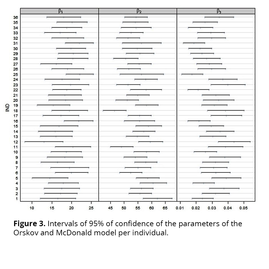
In order to suggest in which parameters it is convenient to include a random effect, the graphs of individual response profiles and of intervals of 95% of confidence were elaborated for each of the parameters of the nonlinear model, using the estimates of the parameters of the adjustments made for all individuals. An unusual variability of the points in some part of the graph of the individual response profiles (at the initial or final points of the process, or on the curvature of the profiles, for instance), associated to some parameter(s) of the nonlinear model chosen, suggests the inclusion of random effect in this/these parameter(s). On the other hand, in the graph of intervals of 95% of confidence, the non-overlap of the intervals calculated for a certain parameter indicates the inclusion of a random effect in this parameter⁽²⁰⁾.

Model (1) with a random effect associated to the rapidly soluble fraction, β1, can be written as:

y_ik = (β_1k + b_1i ) + β_2k[1- exp(-β_3kxi)] + ε_ijκ (4)

in which b1i is the random effect associated to β₁. In this example, it is said that the random effect is linearly associated to the fixed effect parameter β₁, as described by Hist et al.⁽²¹⁾ and Vonesh and Carter⁽²²⁾. If the random effect is associated to the parameter β₂, it is claimed that it will occur linearly. Nevertheless, when a random effect is associated to parameterβ₃ , it will occur nonlinearly, as proposed by Lindstrom and Bates⁽¹⁸⁾.

If these informal techniques of choice of random effects are not conclusive, all possible models can be compared, using likelihood ratio tests (LRT) on embedded models or Akaike's (AIC) or Bayesian (BIC) information criteria, when the models are not embedded. In this case, the model which presented the lowest value of these statistics (AIC or BIC) was considered the most adequate⁽²⁰⁾.

When the model involved more than one random effect, a structure was chosen for matrix D, associated to the vector of random effects, that is parsimonious and can explain well the variability and the covariances among such effects.

For the final model and after the choice of the random effects, distinct mean curves were adjusted for each treatment and the comparisons among the treatments were made as described in Sartorio⁽¹⁴⁾. All analyses were performed using the package nlme of the software R⁽²³⁾, considering a level of significance α=0.05 in all tests of hypothesis.

Results and Discussion

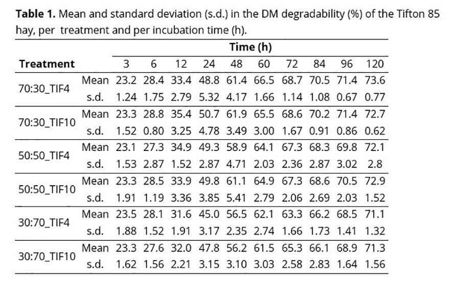
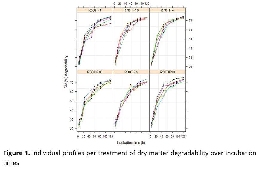
The individual profiles of dry matter (DM) degradability over time, per treatment (Figure 1), have similar behaviors, present some heterogeneity of variances over time and indicate that the nonlinear model (1) can explain well the relation between the percentage of DM degradation and the incubation times.

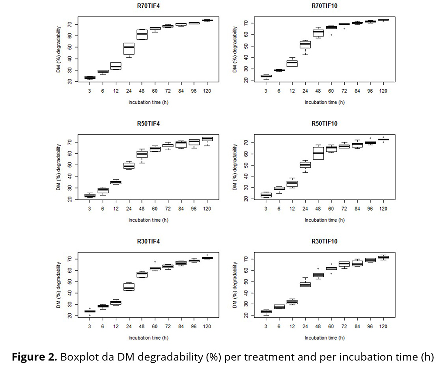
In Table 1, in general, a rise in the variability of the responses is observed until 24 or 48 hours of incubation, with a further decrease until 120 hours, for all treatments, an aspect that is not so evident in the graphs of individual profiles (Figure 1), being more evident in Figure 2.

The model of Orskov and McDonald⁽¹⁶⁾ was adjusted for each of the thirty-six individuals, resulting from the combination of the six animals evaluated at six different periods. For the three response variables studied (estimates of β₁, β₂, and β₃), the Shapiro-Wilk and Bartlett tests confirmed the normality of the errors (p>0.05) and the homogeneity of variances among the six treatments (p>0.05), respectively.

The individual ANOVAs of these response variables indicated that there was no interaction (p >0.05) between the levels of the factors R:C and TIF, that no effect of the TIF factor was observed on DM degradability, with significant differences (p <0.05) occurring only among the means of the levels of factor R:C. These results were in agreement with those obtained by Feitosa et al.^(17).

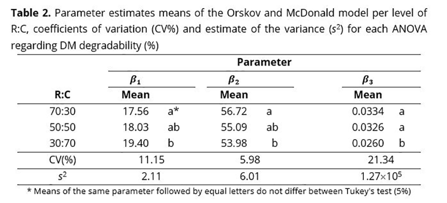
The coefficients of variation (Table 2) were considered medium-high for the parameters β₁ and β₃, and low-medium for the parameter β₂ , according to the classification of Vaz et al.⁽²⁴⁾. By the Tukey's test, it was noticed that the animals which received 70% of roughage in the feed presented a higher value of β₂ and a lower value of than the animals which received only 30% of roughage. The treatments with 70 and 50% of roughage presented mean β3 values equal to each other and superior to that of the treatment with 30% of roughage.

The intervals of 95% of confidence developed for the three parameters from the adjustments of the model for the 36 individual profiles of DM(%) degradability (Figure 3) suggest the inclusion of random effect in β₂, β₃ and, possibly, in β1, since the number of non-overlapping intervals for this parameter is small. To confirm these suggestions, seven models with random effects were suggested (Table 3).

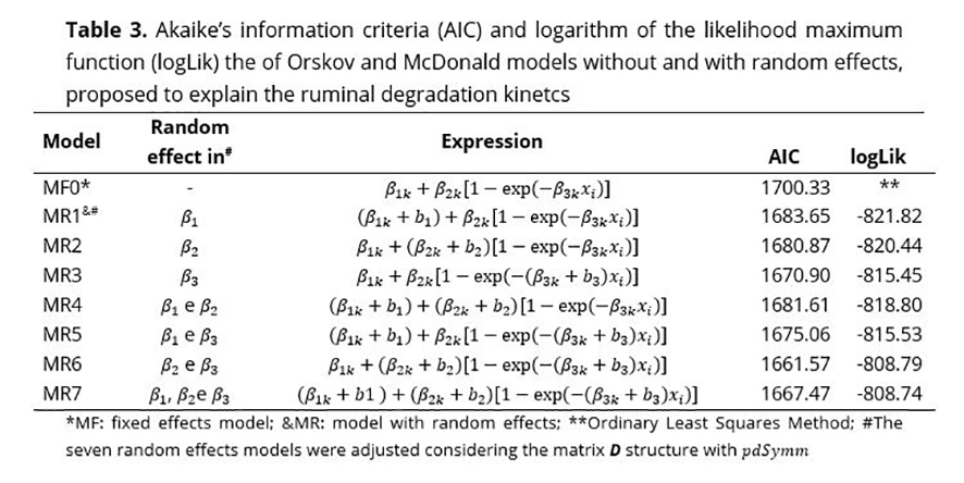
To search for the appropriate structure of variances and covariances for the random effects, the seven models with random effects presented in Table 3 were combined, with four structures for matrix D(pdSymm: general positive-definite matrix, with no additional structure; pdLogChol: general positive-definite matrix, with no additional structure, using a log-Cholesky parameterization; pdDiag: diagonal; pdIdent : multiple of an identity), admitting R_i = σ²In_i .

Likelihood Ratio Tests (LRT) and the criteria AIC and BIC indicated that model MR6, with random effects in β₂ and β₃, with a non-structured matrix for D , provided a better adjustment than the model with fixed effects (MF0) and all other mixed nonlinear models.

The need to use another structure for matrix R (first-order autoregressive – AR(1); first-order autoregressive with heterogeneity of variances – ARH(1) or composed symmetry – CS) was also tested, but the results confirmed that the structure R = σ²I10 is the most appropriate.

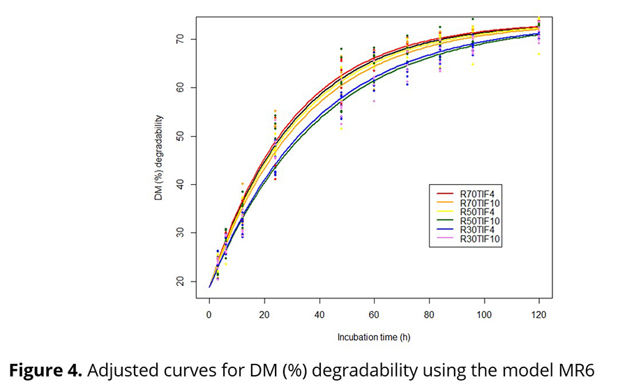
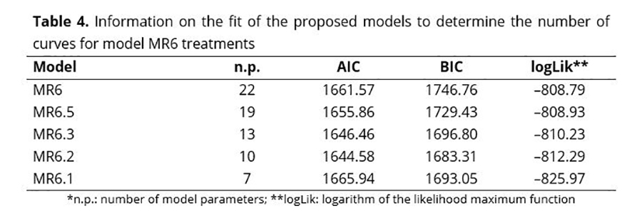
In Figure 4, which presents the mean curves adjusted to the six treatments, it is observed that the curves of treatments R30TIF4 and R30TIF10 are very similar, as well as the curves from the other treatments. Considering the random structure of model MR6 and the mean curves presented, some alternative models were proposed: i) MR6.5: five distinct curves, with a single curve for treatments R30TIF4 and R30TIF10 and one curve for each of the other treatments; ii)MR6.3: three distinct curves, comprising one for treatments R70TIF4 and R70TIF10, another for R50TIF4 and R50TIF10 and another for R30TIF4 and R30TIF10; iii) MR6.2: two distinct curves, one for treatments R30TIF4 and R30TIF10 and the other for the other treatments R70TIF4, R70TIF10, R50TIF4 and R50TIF10; iv) MR6.1: a single curve for all mean profiles. The models were compared using LRT and the criteria AIC and BIC and it was concluded that model MR6.2 with 10 parameters is as good as the other models, which involve 13, 19 or 22 parameters (Table 4). Therefore, the DM (%) degradability curves depending on the incubation times were considered identical for the roughage percentages of 70 and 50, with only the percentage of 30 considered different from the others. The nutritional quality of the Tifton 85 hays (TIF4 and TIF10) did not influence DM (%) degradability.

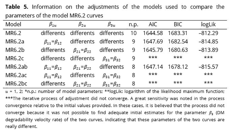
The parameters of model MR6.2 were also compared using the models presented in Table 5. Likelihood ratio tests were performed and allowed the conclusion that model MR6.2 with two curves and distinct parameters was the most indicated for the description of the response variable under study.

Reminding that the random structure of the was selected previously to that of the fixed effects, Pinheiro and Bates⁽²⁰⁾ recommend that the structure of matrix R be confirmed, in other words, whether this structure remains the same chosen before defining the fixed effects. Among the most complex structures (AR(1), ARH(1) and CS) compared, by LRT, with R = σ²I10, structure ARH(1), with different variances at the different incubation times and first-order autocorrelation, was considered the most adequate.

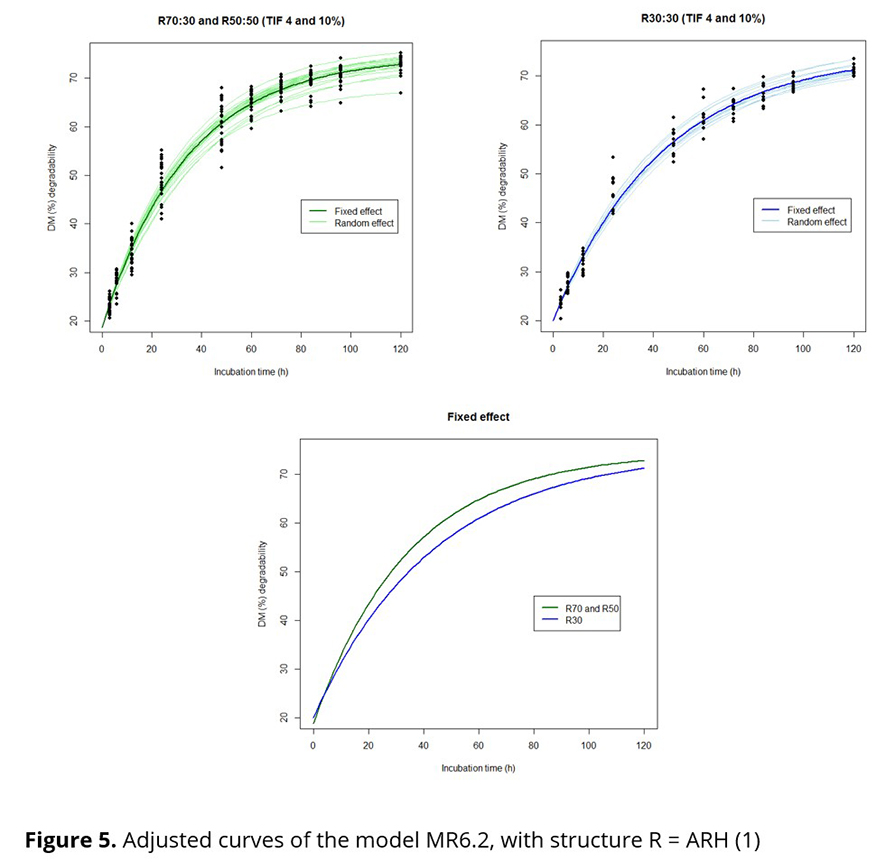
The treatments with 70 or 50% of roughage did not present differences from each other for all parameters of the model, but they were different from the treatments in which the roughage percentage was of 30% (also for all parameters of the model). The final mixed nonlinear model explains virtually all variability present in the data (Figures 5 and 6), which does not occur with the model of two phases.

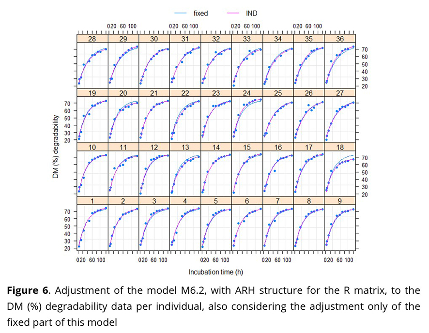
In Figure 6, a very distinct behavior of the responses is observed for individual 18 in relation to the other individuals, presenting the highest variation regarding the potentially degradable fraction (β₂). This fact explains the need for a higher predicted value of the random effect, regarding parameter β₂, found for individual 18.

The lowest proportion of concentrate resulted in a higher DE5% of the Tifton hay, in relation to the other proportions considered. Conversely, the DPs of both treatments presented virtually the same values (Table 6), which were consistent with those obtained by Jobim et al.⁽⁹⁾.

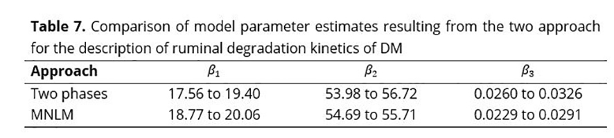
In the two approaches, the roughage percentages 70 and 50 in the feed did not present difference for any of the parameters evaluated, that is, for the rapidly degradable fraction (β₁), for the potentially degradable fraction (β₂) and for the rate of degradation of the potentially degradable fraction (β₃). The values of the estimates of parameters β₁, β₂ and β₃ of the final models of the mixed approach are close to the variation ranges (or to the intervals of variation) obtained with the approach of two phases (Tables 6 and 7), the mixed approach presenting the lowest variation.

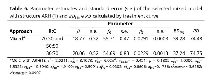
Considering the final model, MR6.2 with structure ARH(1) for matrix R, the lowest proportion of roughage in the feed provided the lowest ED5% of Tifton 85 hay (37.24%), in relation to the other proportions considered, being close to the values found by Assis et al.⁽²⁶⁾, Balieiro and Melloti⁽²⁵⁾, as well as close to the interval of values obtained in the two-phase (37.68 to 40.01) and mixed (37.31 to 40.38) approaches. On the other hand, the PDs of both treatments presented very close values, being also in agreement with those obtained by the two-phase approach (73.12 to 74.28), values close to the obtained by Jobim et al.⁽⁹⁾ and superior to those found by Balieiro and Melloti⁽²⁵⁾. Furthermore, the estimation of the residual variability (s²) referring to the analysis of two phases suffered a great reduction (from 6.84 to 2.02) already expected, since the residual variability, which previously could be explained by a single source of variation in the classic nonlinear model (analysis of two phases), started to be composed of variations among individuals (residual variation plus random effects) and intraindividual (relative to the heterogeneity of variances in the several incubation times) in the mixed nonlinear model, justifying its reduction. Thus, the use of MNLM is better than the method in two phases to differentiate the effective and potential degradability of foods, since, if the standard error of the parameter estimations is higher, the respective intervals of 95% of confidence will also be higher, reducing the probability of finding difference among the treatments, in other words, the probability of erroneously accepting the null-effect hypothesis of the treatments (type II error) increases.

The results regarding the fixed effects obtained with the use of MNLM were not distinct from those obtained in the analysis of two phases, under the conditions of this trial. Nevertheless, the mixed approach presents advantages compared to the approach of two phases, when the interest is in the description of the behavior of the individual response profiles and in the separation of the residual variability in sources of variation among and within individuals.

Similar results were obtained by Zanton and Heinrichs⁽²⁷⁾, who performed a study for the response variable neutral detergent fiber (NDF), in which they evaluated three methodologies for the analyses of food degradation profiles in situ. For this, they simulated 500 experiments, considering only four animals, two periods and eight incubation times (72, 48, 24, 16, 8 ,4, 2, and 1h). Under these conditions, the authors could conclude that, in many cases, MNLM is as good as or better than the analysis of two phases.

The variability caused by the experimental design on the responses was well explained by the structures of covariances used, indicating that the inclusion of parameters related to the design factors is not necessary with the use of the mixed nonlinear model.

Conclusion

The use of the model of Orskov and McDonald⁽¹⁶⁾ with random effects provided the best adjustment for the data on dry matter degradability, since data variability is better described. The package nlme of the software R was very versatile in the adjustment, enabling the adjustment and comparison of several models for the fixed part, alternating several structures of variances and covariances.

The use of mixed nonlinear models in the analysis of data on digestibility in situ is very advantageous when the research aims at understanding the behavior of the digestibility process throughout the incubation times. If the interest is restricted to the estimation of the parameters of the nonlinear model of Orskov and McDonald and to the calculation of the effective and potential degradabilities of the diets, any of the two approaches of analysis presented can be used.

Although this study suggests that, for reducing the estimate of residual variability (s²), the use of MNLM is better than the method in two phases to differentiate the effective and potential degradability of foods, it is necessary to perform simulations to prove such affirmation.

Acknowledgement

To prof. Dr. José Valmir Feitosa for giving in the data. To CAPES for the scholarship. This paper is part of the doctoral thesis of the author's first, obtained by ESALQ/USP.

References